A Physical Modeling Audio Effect
I have been interested in Physical Modeling for some time. The fact that you reach a very similar result in two completely different ways is fascinating. I used a Line6 Pod (the first version) as a guitar amp for a long time and I still think it is fascinating how they managed to get this functionality on some lame ass CPU in 1997.
Twenty years later a freezer has probably more CPU power than the Line6 Pod and there are other possibilities for physical (Amp-)Modeling. Some DAWs have amp modeling built in, there are tons of amp modeling apps for iOS, and there is hardware from all major amp manufacturers and specialists like Kemper, Fractal Audio and Line6 amongst others.
Because the math behind DSP stuff is not easy, I picked a topic where I could check the result. There is a tool for Windows (95!!) that shows the frequency response for common guitar amp tonestacks. I also found this dissertation by David Yeh at Stanford which is a great read if you want to get into the topic. What is a tonestack? It is the EQ section (Low, Mid, Treble) of an amplifier.
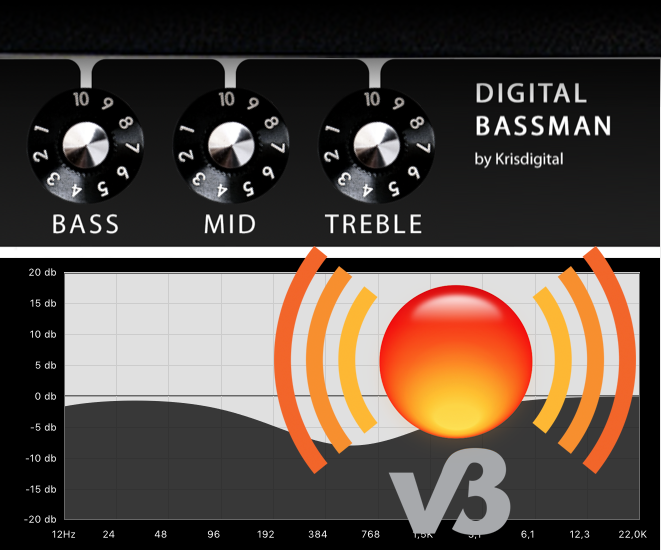
The Fender Bassman is a legendary amplifier introduced in 1952. As many other amps (Marshall amongst others) use the same electrical circuit for their tonestack, you could just change the values of the resistors and capacitors to simulate another amp’s tonestack.
What I did:
- Analyze the circuit
- Calculate the function of the output voltage
- Transfer the equations to the digital domain
- Implement the filter
- Build an AudioUnit Extension
A lot of work to be covered! As a motivation to read on, here is a video of the result (I know, there are some visual incontinuities with the knobs :=)).
What is special about this filter?
- When you turn everything up, there is a mid cut, no flat curve
- There are no independent filter bands, the paramaters influence each other
Analyze the circuit
There is more than one way to analyze a circuit, I chose the technique of nodal analysis. The sum of currents at each node is equal to zero. I marked the nodes as “o” in the diagram.
                 C1

                 + +
Vi  +------+-----+ +-----o  Vex
           |     + +     |
           |            +++
           |            | |
           |            | |  (1-t)*R1
           |            | |
          +++           +++
          | |            +
      R4  | |            o-------+  Vo
          | |            |
          +++            |
           |            +++
           |            | |
           |            | |  t*R1
           |            | |
           |     C2     +++
           |             |
           |     + +     |
           o-----+ +-----o
           |     + +     |
           |             |
           |            +++
           |            | |
           |            | |  l*R2
           |            | |
           |            +++
           |             |
           |             o
           |             +
           |            +++
           |            | |
           |            | |  (1-m)*R3
           |     C3     | |
           |            +++
           |     + +     |
           +-----+ +-----o
                 + +     |
                         |
                        +++
                        | |
                        | |  m*R3
                        | |
                        +++
                         |
                         |
                       +---+
                        +-+
                         +
The current through a capacitor is i = C * dv/dt, so for the voltage Vex in the diagram you will get the following equation:
C1*dv/dt*(Vi-Vex) + (Vo-Vex)/((1-t)*R1) = 0
Repeating this at the other nodes results in six equations for six voltages, we are interested in Vo. One problem are the terms dv/dt, but luckily there is a thing called Laplace Transform that allows you to replace every occurence of dv/dt with an s.
Calculate the function of the output voltage
Still this linear equation system is hard to solve manually. Probably my old TI-89 calculator could have done it, but there is a great open source software called Maxima. It is based on software from 1968 and is still widely used. The only functions I needed were linsolve to solve the equations and ratsimp to factor out variables.
The result for Vo:
Vo = ((C1*R1*Vi*(C2*(C3*R3*R4-C3*R3*R4*m)+C2*C3*R2*R4*l)*s^3+C1*R1*(C3*R4+C2*R4)*Vi*s^2+C1*R1*Vi*s)*t+Vi*
(C1*(C2*(C3*R3^2*R4*m-C3*R3^2*R4*m^2)+C2*C3*R2*R3*R4*l*m)+C1*R1*(C2*(C3*R3^2*m-C3*R3^2*m^2)+C2*C3*R2*R3*l*m))*s^3+Vi*(C1*
(-C3*R3^2*m^2+R2*l*(C3*R3*m+C3*R4+C2*R4)+C3*R3^2*m+C3*R3*R4+C2*R3*R4)+C2*(C3*R3^2*m-C3*R3^2*m^2)+C1*R1*(C3*R3*m+C2*R2*l+C2*R3)+C2*C3*R2*
R3*l*m)*s^2+Vi*(C3*R3*m+C1*(R2*l+R3)+C2*R2*l+C2*R3)*s)/(
(C1*(C2*(C3*R3^2*R4*m-C3*R3^2*R4*m^2)+C2*C3*R2*R3*R4*l*m)+C1*R1*(C2*(-C3*R3^2*m^2+(C3*R3^2-C3*R3*R4)*m+C3*R3*R4)+C2*R2*l*(C3*R3*m+C3*R4)))*s^3+
(C1*(-C3*R3^2*m^2+R2*l*(C3*R3*m+C3*R4+C2*R4)+C3*R3^2*m+C3*R3*R4+C2*R3*R4)+C2*(-C3*R3^2*m^2+(C3*R3^2-C3*R3*R4)*m+C3*R3*R4)+C1*R1*
(C3*R3*m+C2*R2*l+C2*(R4+R3)+C3*R4)+C2*R2*l*(C3*R3*m+C3*R4))*s^2+(C3*R3*m+C1*(R2*l+R3)+C2*R2*l+C2*(R4+R3)+C3*R4+C1*R1)*s+1)
😳
Transfer the equations to the digital domain
For a filter we need the transfer function
H(s) = Vo/Vi
Easily enough that just removes all occurrences of Vi in our equation for Vo.
For implementing the filter later we need to transform this to be of the form:
         b0 + b1*z^-1 + b2*z^-2 + b3*z^-3
H(z) = ------------------------------------
         1 + a1*z^-1 + a2*z^-2 + a3*z^-3
For that the bilinear transform is used. We set s = K*(1-z)/(1+z) and I used ratsimp
in Maxima like ratsimp(Vo, z) to get the coefficients b0, b1, b2, b3 and a1, a2, a3. K is 1/T where T is the time interval between the digital samples, for example 1/44100 seconds.
H(z) = (((C1*C2*C3*K^3*R1*R3*R4*m-C1*C2*C3*K^3*R1*R2*R4*l+(((-C1*C3-C1*C2)*K^2*R1-C1*C2*C3*K^3*R1*R3)*R4-C1*K*R1))*t+
(C1*C2*C3*K^3*R3^2*R4+(C1*C2*C3*K^3*R1+(C2+C1)*C3*K^2)*R3^2)*m^2+((((-C2-C1)*C3*K^2-C1*C2*C3*K^3*R1)*R2*R3-C1*C2*C3*K^3*R2*R3*R4)*l+
(-C1*C2*C3*K^3*R3^2*R4+((-C2-C1)*C3*K^2-C1*C2*C3*K^3*R1)*R3^2+(-C1*C3*K^2*R1-C3*K)*R3))*m+
((-C1*C3-C1*C2)*K^2*R2*R4+((-C2-C1)*K-C1*C2*K^2*R1)*R2)*l+((-C1*C3-C1*C2)*K^2*R3*R4+((-C2-C1)*K-C1*C2*K^2*R1)*R3))*z^3+(
(-3*C1*C2*C3*K^3*R1*R3*R4*m+3*C1*C2*C3*K^3*R1*R2*R4*l+((3*C1*C2*C3*K^3*R1*R3+(C1*C3+C1*C2)*K^2*R1)*R4-C1*K*R1))*t+
(((-C2-C1)*C3*K^2-3*C1*C2*C3*K^3*R1)*R3^2-3*C1*C2*C3*K^3*R3^2*R4)*m^2+((3*C1*C2*C3*K^3*R2*R3*R4+(3*C1*C2*C3*K^3*R1+(C2+C1)*C3*K^2)*R2*R3)*l+
(3*C1*C2*C3*K^3*R3^2*R4+(3*C1*C2*C3*K^3*R1+(C2+C1)*C3*K^2)*R3^2+(C1*C3*K^2*R1-C3*K)*R3))*m+
((C1*C3+C1*C2)*K^2*R2*R4+(C1*C2*K^2*R1+(-C2-C1)*K)*R2)*l+((C1*C3+C1*C2)*K^2*R3*R4+(C1*C2*K^2*R1+(-C2-C1)*K)*R3))*z^2+(
(3*C1*C2*C3*K^3*R1*R3*R4*m-3*C1*C2*C3*K^3*R1*R2*R4*l+(((C1*C3+C1*C2)*K^2*R1-3*C1*C2*C3*K^3*R1*R3)*R4+C1*K*R1))*t+
(3*C1*C2*C3*K^3*R3^2*R4+(3*C1*C2*C3*K^3*R1+(-C2-C1)*C3*K^2)*R3^2)*m^2+((((C2+C1)*C3*K^2-3*C1*C2*C3*K^3*R1)*R2*R3-3*C1*C2*C3*K^3*R2*R3*R4)*l+
(-3*C1*C2*C3*K^3*R3^2*R4+((C2+C1)*C3*K^2-3*C1*C2*C3*K^3*R1)*R3^2+(C1*C3*K^2*R1+C3*K)*R3))*m+
((C1*C3+C1*C2)*K^2*R2*R4+(C1*C2*K^2*R1+(C2+C1)*K)*R2)*l+((C1*C3+C1*C2)*K^2*R3*R4+(C1*C2*K^2*R1+(C2+C1)*K)*R3))*z+
(-C1*C2*C3*K^3*R1*R3*R4*m+C1*C2*C3*K^3*R1*R2*R4*l+((C1*C2*C3*K^3*R1*R3+(-C1*C3-C1*C2)*K^2*R1)*R4+C1*K*R1))*t+
(((C2+C1)*C3*K^2-C1*C2*C3*K^3*R1)*R3^2-C1*C2*C3*K^3*R3^2*R4)*m^2+((C1*C2*C3*K^3*R2*R3*R4+(C1*C2*C3*K^3*R1+(-C2-C1)*C3*K^2)*R2*R3)*l+
(C1*C2*C3*K^3*R3^2*R4+(C1*C2*C3*K^3*R1+(-C2-C1)*C3*K^2)*R3^2+(C3*K-C1*C3*K^2*R1)*R3))*m+
((-C1*C3-C1*C2)*K^2*R2*R4+((C2+C1)*K-C1*C2*K^2*R1)*R2)*l+((-C1*C3-C1*C2)*K^2*R3*R4+((C2+C1)*K-C1*C2*K^2*R1)*R3))/((
(C1*C2*C3*K^3*R3^2*R4+(C1*C2*C3*K^3*R1+(C2+C1)*C3*K^2)*R3^2)*m^2+((((-C2-C1)*C3*K^2-C1*C2*C3*K^3*R1)*R2*R3-C1*C2*C3*K^3*R2*R3*R4)*l+
((C1*C2*C3*K^3*R1+C2*C3*K^2)*R3-C1*C2*C3*K^3*R3^2)*R4+((-C2-C1)*C3*K^2-C1*C2*C3*K^3*R1)*R3^2+(-C1*C3*K^2*R1-C3*K)*R3)*m+
((((-C2-C1)*C3-C1*C2)*K^2-C1*C2*C3*K^3*R1)*R2*R4+((-C2-C1)*K-C1*C2*K^2*R1)*R2)*l+
((((-C2-C1)*C3-C1*C2)*K^2-C1*C2*C3*K^3*R1)*R3+(-C1*C3-C1*C2)*K^2*R1+(-C3-C2)*K)*R4+((-C2-C1)*K-C1*C2*K^2*R1)*R3-C1*K*R1-1)*z^3+(
(((-C2-C1)*C3*K^2-3*C1*C2*C3*K^3*R1)*R3^2-3*C1*C2*C3*K^3*R3^2*R4)*m^2+((3*C1*C2*C3*K^3*R2*R3*R4+(3*C1*C2*C3*K^3*R1+(C2+C1)*C3*K^2)*R2*R3)*l+
(3*C1*C2*C3*K^3*R3^2+(-3*C1*C2*C3*K^3*R1-C2*C3*K^2)*R3)*R4+(3*C1*C2*C3*K^3*R1+(C2+C1)*C3*K^2)*R3^2+(C1*C3*K^2*R1-C3*K)*R3)*m+
((3*C1*C2*C3*K^3*R1+((C2+C1)*C3+C1*C2)*K^2)*R2*R4+(C1*C2*K^2*R1+(-C2-C1)*K)*R2)*l+
((3*C1*C2*C3*K^3*R1+((C2+C1)*C3+C1*C2)*K^2)*R3+(C1*C3+C1*C2)*K^2*R1+(-C3-C2)*K)*R4+(C1*C2*K^2*R1+(-C2-C1)*K)*R3-C1*K*R1-3)*z^2+(
(3*C1*C2*C3*K^3*R3^2*R4+(3*C1*C2*C3*K^3*R1+(-C2-C1)*C3*K^2)*R3^2)*m^2+((((C2+C1)*C3*K^2-3*C1*C2*C3*K^3*R1)*R2*R3-3*C1*C2*C3*K^3*R2*R3*R4)*l+
((3*C1*C2*C3*K^3*R1-C2*C3*K^2)*R3-3*C1*C2*C3*K^3*R3^2)*R4+((C2+C1)*C3*K^2-3*C1*C2*C3*K^3*R1)*R3^2+(C1*C3*K^2*R1+C3*K)*R3)*m+
((((C2+C1)*C3+C1*C2)*K^2-3*C1*C2*C3*K^3*R1)*R2*R4+(C1*C2*K^2*R1+(C2+C1)*K)*R2)*l+
((((C2+C1)*C3+C1*C2)*K^2-3*C1*C2*C3*K^3*R1)*R3+(C1*C3+C1*C2)*K^2*R1+(C3+C2)*K)*R4+(C1*C2*K^2*R1+(C2+C1)*K)*R3+C1*K*R1-3)*z+
(((C2+C1)*C3*K^2-C1*C2*C3*K^3*R1)*R3^2-C1*C2*C3*K^3*R3^2*R4)*m^2+((C1*C2*C3*K^3*R2*R3*R4+(C1*C2*C3*K^3*R1+(-C2-C1)*C3*K^2)*R2*R3)*l+
(C1*C2*C3*K^3*R3^2+(C2*C3*K^2-C1*C2*C3*K^3*R1)*R3)*R4+(C1*C2*C3*K^3*R1+(-C2-C1)*C3*K^2)*R3^2+(C3*K-C1*C3*K^2*R1)*R3)*m+
((C1*C2*C3*K^3*R1+((-C2-C1)*C3-C1*C2)*K^2)*R2*R4+((C2+C1)*K-C1*C2*K^2*R1)*R2)*l+
((C1*C2*C3*K^3*R1+((-C2-C1)*C3-C1*C2)*K^2)*R3+(-C1*C3-C1*C2)*K^2*R1+(C3+C2)*K)*R4+((C2+C1)*K-C1*C2*K^2*R1)*R3+C1*K*R1-1)
😳😳
As you can see this rather simple electrical circuit results in a good chunk of mathematical operations in the digital domain!
Note that I did not normalize the equation at this point so that there is a 1+a1... in the denominator, I did it later in the implementation by dividing all parameters.
Calculate the magnitude of the transfer function
For the visualization of the transfer function we need the magnitude as a function of the frequency. For stable systems like our filter we can set z=e^-jw, here is a good explanation for that. With e^-jw = cos(w) - jsin(w) we can put that in the equation of our transfer function and then calculate the magnitude for the nominator and denominator by M1 = sqrt(Real^2 + Imaginary^2), so that the final magnitude is
      Mnominator
M = --------------
     Mdenominator
A good way to check your results is using Python. There a great packages for doing signal processing and visualizations. To plot the frequency response of a digital filter you can use the scipy.signal.freqz function.
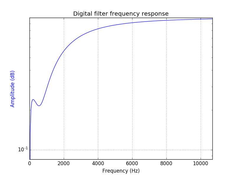 Filter magnitude response for l=0, m=0, t=1
Implement the filter
At this point we have everything we need to implement the digital IIR filter. Actually it is fairly simple to implement, all you need to do is put the coefficients in the following equation:
(b0 * x0) + (b1 * state.x1) + (b2 * state.x2) + (b3 * state.x3) - (a1 * state.y1) - (a2 * state.y2) - (a3 * state.y3)
Where state contains past values, so state.x1 is x[n-1] etc.
The theory behind that is shown in this illustration.
Extra: Build an AudioUnit Extension
At first I built this as an AudioUnitV3. I saw a presentation of the new technology and one of the code examples was an EQ, so it was a good starting point for prototyping. You can skip this as I ported the effect to VST3/AU in the meantime!
First off, what is an AudioUnit Extension. To be honest when I started this I thought it would just be the next version of AudioUnits, but it is a completly different concept, that Apple does not only use for Audio but for all kinds of stuff. I started with the example code which already includes a filter example, which comes handy.
App extensions always have to be embedded in an app, that is how they are distributed. The reason behind that is probably iOS and the app store: you need an app to get new software on iDevice. So when you launch the app, the contained AppExtension is registered and can then be used as usually.
I developed a macOS Audio Extension because I wanted to use it in Logic9 and Garageband, but I realized that is not supported yet. It does not even work in AU Lab either. There comes an AuV3ExampleHost with the example code that you can use. I will probably try to extract the audio unit and compile a good old AudioUnit so that I can share it more easily and use it myself. The newest Logic should support them, that is what I heard at least..
The example code has a pretty complex build setup to show you how to build the effect for iOS and macOS while reusing common framework code. If you start from scratch there is a template for the AudioUnit Extension build target.
But what I did is just to modify the appropriate functions in FilterDSPKernel.hpp, that is where the processing takes place. And of course the parameters have to be rewired.
User Interface
If you want an App Extension that runs on iOS and macOS you can only reuse the processing code, not the UI. iOS uses UIKit, macOS uses AppKit. They are similar, but still you cannot just reuse the UI-code and Interface-Builder files. For example in AppKit there is a circular slider element (=Knob), in UIKit there isn’t. While on iOS you will use UIClassName, on macOS it will be NSClassName etc.
For the filter I just needed some Knobs as a control for the parameters Low, Mid and Treble. For that I made a custom NSControl element. What I learned here is the use of @IBDesignable and @IBInspectable to actually see the element in interface builder (IB) to tweak it:
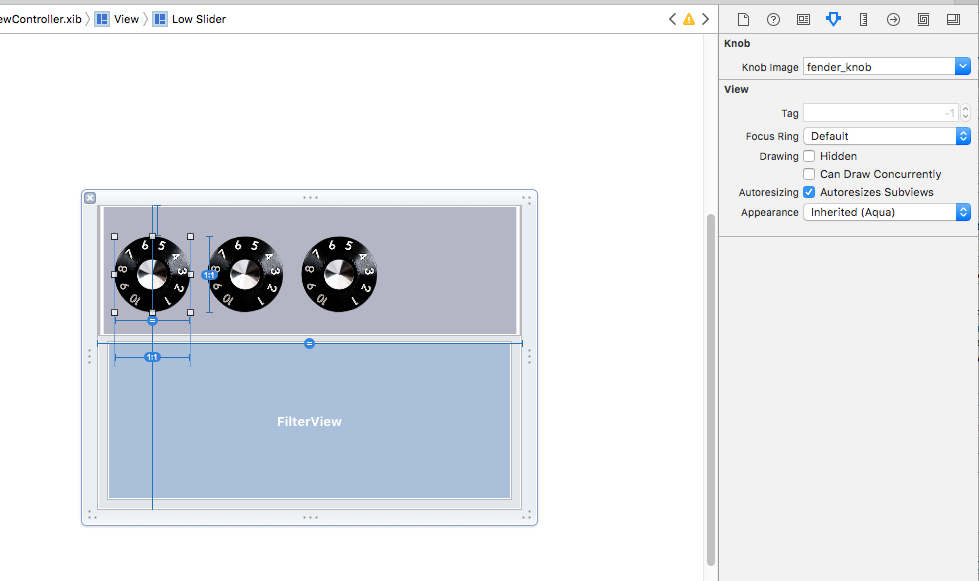 As you can see you can select an image for the knob in IB and it is rendered in the preview.
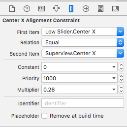
Another thing is responsive design. As your extension might run on all kinds of devices, it is important that it behaves well on the different screen sizes. For that Autolayout is probably the way to go as it is here to stay. Even if I think the term ‘Autolayout’ is somewhat an euphemism :=)
To get the knobs scale relatively to the superview and to keep their position I used the following approach of aligning the centers and using a multiplier. 0 is left, 1 is middle, and 2 is right. Then I made the width of the knob a fraction of the superview width and the aspect ratio 1:1 et voilà..
Download
In the meantime I ported the plugin to VST/AU!